


Quantifying the Transformation of Chokepoints in Modern Networked Interdependence
Introduction
Historically, strategic chokepoints were defined by their physical geography, with maritime corridors like Malacca or the Suez Canal concentrating critical economic and material flows into narrow, constrained paths, granting controllers coercive leverage through potential disruption. However, modern interdependence has decoupled vulnerability in systemic structures from physical topography. Global production networks distribute activities across transnational jurisdictions, while concentrating critical functions, from critical mineral processing to semiconductor manufacturing, into highly specialised nodes, creating severe bottlenecks despite being embedded within a system of dispersed and interdependent supply chains.
Such nodes become bottlenecks when dependence on their output, combined with limited substitutability and bypassing capacity, gives actors the capability to impose disproportionate costs on network participants. This shift poses a fundamental question: if the leverage of a traditional chokepoint derives entirely from its structural position within a broader interdependent network, can economic and technological nodes generate identical power when occupying equivalent positions?
Theoretical Framework
Keohane and Nye’s complex interdependence theory challenges the realist ontologies of the international system as centred on states and military security (Keohane & Nye, 1977). Their theory, instead, recognises multiple channels connecting societies, including interstate, transgovernmental and transnational relations, through which states, firms and other actors transmit effects across borders. As domestic and foreign policies become increasingly entwined, economic systems consequently become more consequential theatres of international relations. Yet, interdependence does not imply symmetric dependence. Keohane and Nye distinguish between sensitivity, the liability to suffer costs imposed by external events before policy adjustment can occur, and vulnerability, or the enduring costs actors continue to bear after adjustment or adaptation is exhausted. Vulnerability, consequently, depends on the availability and cost of alternatives, wherein an actor may be highly sensitive to disruption yet comparatively less vulnerable if alternatives can be established readily, while dependence becomes consequential when adjustment is costly, slow, or insufficient.
Global production networks conceptualise production as geographically extensive configurations of interconnected firms, functions and institutions that transcend organisational & national boundaries (Hendorson et al., 2002). Yet geographic extension does not entail an equitable distribution of productive capacity. Instead, GPNs are territorially embedded within institutional and economic configurations of certain locations, wherein accumulated local relationships and capabilities generate spatial lock-in, and their embeddedness is conditioned by the architecture, durability and stability of inter-actor relations. Krugman’s economic geography supplies a mechanism for the persistence of such concentration through agglomeration (Krugman, 1991), which generates external economies through pooled specialised labour, localised specialised inputs and informational spillovers, while proximity to markets & suppliers lowers transport costs. Under increasing returns, these advantages become cumulative, such that the concentration of purchasing power and intermediate power attracts mobile factors, reinforcing the market and supplier structures that generated this initial advantage, such that this accumulation can create specialised capabilities that become increasingly difficult to reproduce elsewhere, leading to functional concentration. When such concentrated capabilities occupy nodes through which substantial volumes of network activity are mediated, territorial agglomeration acquires a structural dimension, wherein disruption to the node cannot be readily absorbed through substitution, but necessitates costly rerouting, reorganisation & adjustment across actors.
Such chokepoints derive asymmetric power from the network position of actors controlling central intermediary nodes, wherein flows between otherwise connected actors are concentrated through a particular node; control over said node confers the capacity to regulate, restrict, and terminate such flows (Farrell & Newman, 2019). The flow magnitude is consequential since centrality alone establishes positional capacity, while the volume of flows subject to that position determines the potential significance of its disruption. This position generates structural dependence where the chokepoint is difficult to substitute, and actors depend upon it when alternative pathways are absent, limited, or costly relative to the existing connection. Non-substitutability consequently determines whether control over a central node can impose asymmetric adjustment costs, wherein the controller can restrict access while dependent actors cannot readily preserve equivalent connectivity through alternate pathways. Crucially, this dependence is produced by network topology rather than physical or geographic proximity. This framework establishes that dependence should be observable in the topology of networks through which interdependent flows are organised. Chokepoint potential should, thus, emerge where a node occupies an intermediary position between connected nodes, mediates substantial flows, and possesses limited substitutability, regardless of its geographic boundaries. The empirical analysis therefore measures chokepointness as a property of network position, flow concentration, and structural dependence, rather than as an inherent characteristic of particular locations.
Quantitative Analyses & Findings
To identify potential chokepoints, the analysis examines two dimensions of network vulnerability: network concentration and structural centrality. Concentration is measured through the Herfindahl-Hirschman Index (or HHI), calculated from the participation shares of nodes in the relevant supply, production, or processing, thereby capturing the extent to which a network is dependent upon limited participants. Centrality is measured through betweenness centrality, capturing the extent to which a node lies on shortest paths connecting others. Their combination permits distinction between concentration and node-level importance, while identifying configurations where both forms of dependence coincide.
The analysis examines three classes of networks through which interdependence may be structured. The geographic network is constructed from the IMF PortWatch Port-Level Impact dataset, covering 2024-26 and capturing relationships within the global maritime system at the port-and-passage level (International Monetary Fund [IMF] & University of Oxford, 2024), representing a partial year. Similarly, the resource and technological networks are constructed from the BACI international bilateral trade dataset (CEPII, 2025), covering 2022-24, with observations filtered to the relevant product classifications. Here, 2024 is the only year common to both datasets. This temporal difference limits direct comparison across networks, but does not preclude comparison of their structural patterns, as the analysis focuses on network concentration and centrality rather than year-specific changes in these measures. The resource network comprises selected products, while the semiconductor network is defined through HS 8541 (semiconductor devices), 8542 (electronic circuits), and 8486 (semiconductor machinery). Across the networks, observed relationships are represented as weighted and directed flows, providing the basis for calculating concentration and node-level centrality.
The geographic network is relatively unconcentrated overall, with a network HHI of only 691.2, indicating that maritime activity is broadly distributed across nodes. Yet structural vulnerability remains uneven, with Korea and Bohai, despite substantial HHI contributions (129.46 and 78.88), recording zero betweenness centrality, demonstrating that traffic concentration alone does not confer chokepoint capacity. Conversely, Suez combines low concentration (7.52) with meaningful centrality (0.187), indicating importance disproportionate to its traffic.
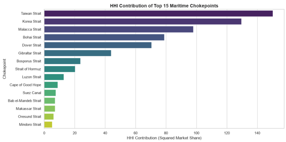
Figure 1: Individual HHI contributions of top maritime chokepoints, demonstrating localised market concentration
Malacca and Taiwan represent the strongest convergence, combining high HHIs (98.01 and 150.15) with the network’s highest betweenness centralities (0.626 and 0.592). These results reveal a crucial distinction between distributions of activity and vulnerability: resilience at the aggregate level (low network HHI) can coexist with positional dependence at the node level.

Figure 2: Betweenness centrality across distance functions, highlighting Malacca and Taiwan’s structural dominance
The mineral network reveals a structurally concentrated form of interdependence where vulnerability is shaped by both aggregate concentration and positional asymmetry. With a network HHI of 1,598.7, activity is substantially concentrated, while the distribution of centrality does not mirror this concentration. China holds the largest network share (15.66%) but ranks third in betweenness centrality (0.413), while India accounts for only 1.33% of the activity yet ranks fourth in centrality (0.271). Conversely, Indonesia ranks fifth in trade activity but records negligible centrality (0.004). The network, thus, reveals that concentrated interdependence does not produce uniform structural power. Instead, vulnerability depends not only on trade activity but on who occupies positions capable of connecting and mediating flows.

Figure 3: Comparison of the top 15 critical-mineral processing countries by betweenness centrality and total trade activity ($US billion)
The semiconductor network reveals a highly asymmetric form of functional interdependence, where a small number of nodes account for a disproportionate share of both centrality and concentration. China combines the largest participation ($498.7 billion) with a weighted centrality of 0.853, more than twice that of the US (0.343) and over thrice that of Germany (0.232). Yet substantial participation does not translate into structural centrality, where Japan participates in $113.1 billion of network activity but records only 0.027 betweenness, while Singapore combines $195.4 billion in participation with a substantial centrality of 0.1666. The network, thus, reveals that semiconductor interdependence is structured through pronounced positional asymmetries, where particular economies can acquire disproportionate capacity to mediate flows irrespective of their absolute participation.

Figure 4: Comparison of the top 15 semiconductor economies by weighted betweenness centrality and gross network participation ($US billion)
Taken together, the three networks suggest a broadening in the locus of strategic chokepoint power from physical geography toward resource and technological networks. Within the geographic network, vulnerability is concentrated around physically constrained nodes such as Malacca and Taiwan, which record the highest betweenness centralities in that network (0.626 and 0.592, respectively), despite its relatively low overall concentration (HHI = 691.2). Within the critical-minerals network, the United States records the highest betweenness centrality (0.557), while the network exhibits the highest aggregate concentration (HHI = 1,598.7). Within the semiconductor network, China occupies the highest betweenness position (0.853), despite an intermediate level of aggregate concentration (HHI = 1,005.3).
The relevant comparison is therefore not between the raw betweenness scores across networks, but between the location and form of their most strategically central nodes: geographic chokepoints in maritime space, resource chokepoints in critical-mineral supply, and technologically embedded chokepoints in semiconductor networks. This pattern is consistent with a broadening of strategic chokepoint power beyond physical geography toward control over critical resources and technological networks.
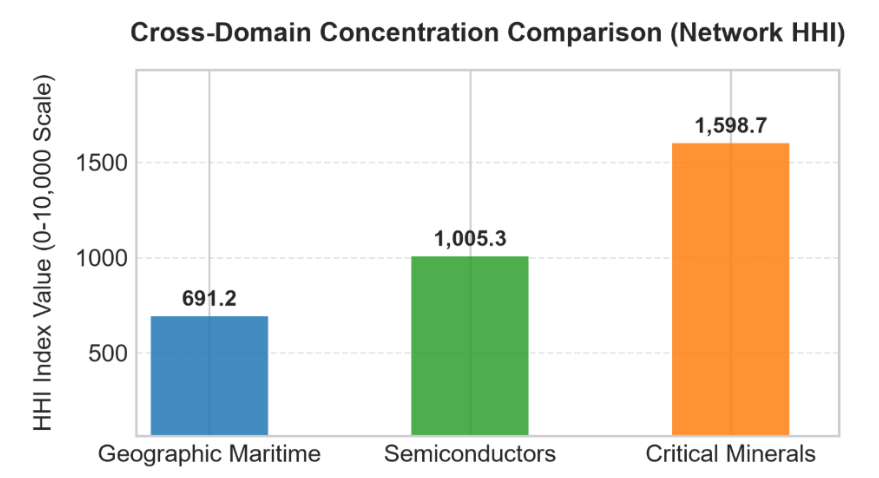
Figure 5: Comparative bar chart of market-share HHI concentration across the geographic, critical-mineral, and semiconductor networks
The contrast demonstrates that chokepoint vulnerability is not reducible to aggregate concentration. Rather, it increasingly emerges from where dependence is located: first in geographically fixed corridors, then in strategic resource networks, and increasingly in specialised technological positions embedded within global production networks.

Figure 6: Cumulative network Betweenness Centrality Pareto distribution comparing geographic, critical-mineral, and semiconductor trade topologies
Conclusion
This study demonstrates that chokepoint vulnerability is fundamentally a function of network structure rather than geography alone. Across maritime, critical-mineral, and semiconductor networks, structural dependence manifests through geographically fixed corridors, concentrated strategic resources, and specialised technological functions. By combining HHI with betweenness centrality, the analysis demonstrates that participation and positional importance can diverge substantially. As global interdependence becomes increasingly embedded within complex production networks, strategic chokepoints therefore extend beyond physical geography into the resource and technological structures underlying the global economy.
References
CEPII. (2025). BACI: International trade database (HS22 version V202501) [Data set]. https://www.cepii.fr/CEPII/en/bdd_modele/bdd_modele_item.asp?id=37
Farrell, H., & Newman, A. L. (2019). Weaponized interdependence: How global economic networks shape state coercion. International Security, 44(1), 42–79. https://doi.org/10.1162/isec_a_00351
Henderson, J., Dicken, P., Hess, M., Coe, N., & Yeung, H. W.-C. (2002). Global production networks and the analysis of economic development. Review of International Political Economy, 9(3), 436–464. https://doi.org/10.1080/09692290210150842
International Monetary Fund & University of Oxford. (2024). PortWatch port-level impact dataset [Data set]. IMF PortWatch. https://portwatch.imf.org/
Keohane, R. O., & Nye, J. S. (1977). Power and interdependence: World politics in transition. Little, Brown.
Krugman, P. (1991). Geography and trade. MIT Press.
Appendix
A. Geographic Network Specification
The geographic network represents maritime interdependence at the port-and-passage level. Each node represents a geographic maritime location, while observed vessel activity constitutes the network flow.
For each node i, total network activity is defined as:
\(S_i = V_i \tag{1}\)
where \(V_i\) denotes the total vessel activity associated with node \(i\).
The participation share of node \(i\) is calculated as:
\(p_i = \frac{V_i}{\sum_{j=1}^{N} V_j} \tag{2}\)
Network concentration is subsequently measured using the Herfindahl-Hirschman Index (HHI):
\(HHI = \sum_{i=1}^{N} p_i^2 \tag{3}\)
For the weighted network representation, bilateral maritime flow between nodes \(i\) and \(j\) is represented by \(V_{ij}\). The corresponding network distance is defined as the inverse of observed flow:
\(d_{ij} = \frac{1}{V_{ij}} \tag{4}\)
Thus, larger observed flows correspond to shorter effective distances within the weighted network.
B. Critical-Mineral Network Specification
The critical-mineral network represents bilateral trade relationships between countries for the selected critical-mineral products. Each country constitutes a node, while bilateral trade constitutes the weighted and directed network flow.
For each country \(i\), gross network participation is defined as the sum of exports and imports:
\(S_i = X_i + M_i \tag{5}\)
where \(X_i\) denotes total critical-mineral exports of country \(i\) and \(M_i\) denotes total critical-mineral imports.
The participation share of country \(i\) is therefore:
\(p_i = \frac{X_i+M_i}{\sum_{j=1}^{N}(X_j+M_j)} \tag{6}\)
Network concentration is measured using:
\(HHI = \sum_{i=1}^{N} p_i^2 \tag{7}\)
For bilateral trade between countries \(i\) and \(j\), trade flow is represented by \(T_{ij}\). The corresponding network distance is:
\(d_{ij} = \frac{1}{T_{ij}} \tag{8}\)
where larger bilateral trade flows produce shorter effective distances within the network.
C. Semiconductor Network Specification
The semiconductor network represents bilateral trade relationships across semiconductor-related products. Countries constitute the nodes, while bilateral trade values constitute the weighted and directed network flows.
The semiconductor network is constructed using the following Harmonized System classifications:
Table 1: Product classifications used in the semiconductor network
HS Code | Product classification |
8541 | Semiconductor devices |
8542 | Electronic integrated circuits |
8486 | Machinery and apparatus used in the manufacture of semiconductor devices |
For each country \(i\), gross semiconductor network participation is defined as:
\(S_i = X_i + M_i \tag{9}\)
where \(X_i\) represents total semiconductor exports and \(M_i\) represents total semiconductor imports.
The participation share of country \(i\) is:
\(p_i = \frac{S_i}{\sum_{j=1}^{N} S_j} \tag{10}\)
Network concentration is measured through:
\(HHI = \sum_{i=1}^{N} p_i^2 \tag{11}\)
For bilateral semiconductor trade \(T_{ij}\) between countries \(i\) and \(j\), the weighted network distance is defined as:
\(d_{ij} = \frac{1}{T_{ij}} \tag{12}\)
This formulation treats stronger bilateral trade relationships as shorter effective distances within the network.
D. Betweenness Centrality
Betweenness centrality measures the extent to which a node occupies an intermediary position on shortest paths connecting other nodes.
For a node \(v\), betweenness centrality is defined as:
\(BC(v) = \sum_{\substack{s \ne v \ne t\\s \ne t}} \frac{\sigma_{st}(v)}{\sigma_{st}} \tag{13}\)
where \(\sigma_{st}\) denotes the number of shortest paths between nodes \(s\) and \(t\), while \(\sigma_{st}(v)\) denotes the number of those paths passing through node \(v\).
For the weighted networks used in this study, shortest paths are determined according to the network-specific distance function defined in the preceding sections. In the trade networks, this distance is based on the inverse of observed bilateral trade:
\(d_{ij} = \frac{1}{T_{ij}} \tag{14}\)
Consequently, stronger bilateral trade relationships correspond to shorter effective network distances, and betweenness centrality captures the extent to which an actor occupies intermediary positions under this weighting structure.
E. Centrality Distribution and Log Transformation
Betweenness centrality exhibits substantial variation across the networks examined in this study. To examine the distribution of centrality and facilitate comparison across observations, both the original and logarithmically transformed measures are considered.
The logarithmic transformation is represented generally as:
\(BC_{log,i} = log(BC_i) \tag{15}\)
where \(BC_i\) denotes the betweenness centrality of node \(i\).
If zero-valued observations are present, the transformation must incorporate the same positive adjustment used in the empirical calculation:
\(BC_{log,i} = log(BC_i + \epsilon) \tag{16}\)
where \(\epsilon > 0\) is the specified adjustment.
The figures below plot the distribution of betweenness centrality across all nodes within each network. Each observation corresponds to a single node, with its position on the horizontal axis reflecting the rank of that node and its position on the vertical axis reflecting the centrality value on the transformed scale described above. The distributions exhibit the pronounced right skew typical of betweenness centrality in sparse weighted networks, in which a small number of nodes occupy highly intermediary positions while the majority record negligible centrality. This skew is precisely what motivates the logarithmic transformation, which compresses the upper tail and permits the full distribution to be examined without the largest values dominating the visual field.
Across the three figures, the shape of the distribution differs markedly: the critical-mineral and semiconductor networks display longer tails and greater dispersion than the geographic network, consistent with the higher aggregate concentration observed at the network level. These distributions provide the basis for the node-level comparisons discussed in the main text, where the gap between a node’s participation share and its centrality rank identifies the structural asymmetry on which the analysis rests.
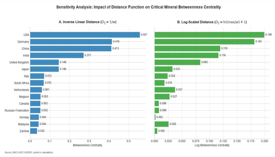
Figure 1A: Betweenness centrality distribution across the critical-mineral network.
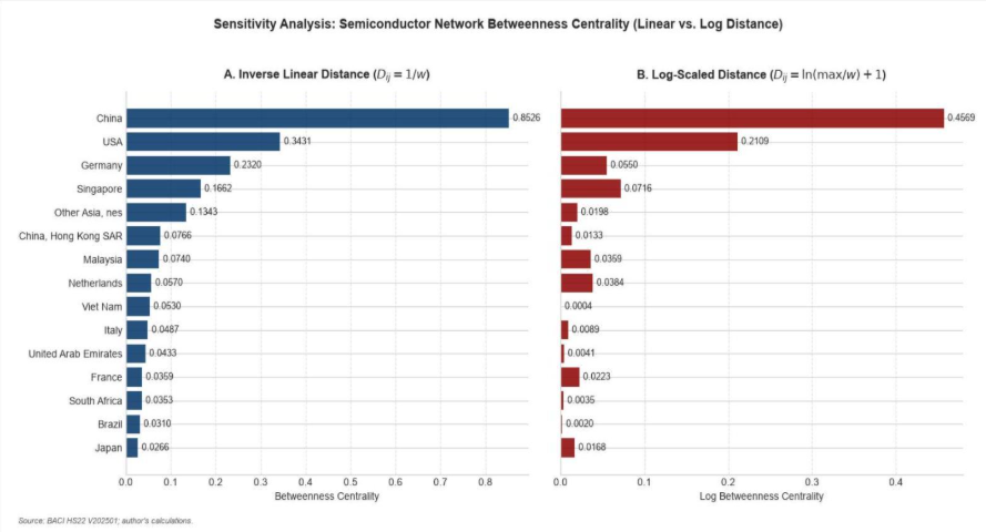
Figure 2A: Betweenness centrality distribution across the semiconductor network.
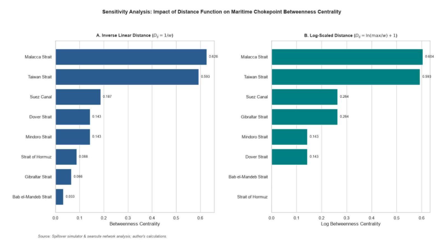
Figure 3A: Betweenness centrality distribution across the geographic network.